Are you intrigued by the generative models, and curious about how they can create new, realistic data? You're in the right place! Today, we're going to explore an exciting class of generative models known as Diffusion Models. We'll unravel the mathematics behind them and then code a basic implementation using PyTorch Lightning.

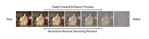
Image reference: twitter.com/iScienceLuvr/status/15648477240..

Demystifying Diffusion Models

Let's first get acquainted with the concept. Diffusion models, as the name suggests, borrow ideas from the natural world, specifically the diffusion process observed in Brownian motion (think of how smoke diffuses in the air or how a drop of ink spreads in water).

In the context of generative modeling, diffusion models start with something simple, like random noise, and gradually refine it to create complex data, like an image or a piece of text. In other words, they start from a simple distribution (like Gaussian noise) and follow a specific path defined by a stochastic differential equation (SDE) to reach the final data distribution. It's like an artist starting with a blank canvas and then meticulously adding strokes until a masterpiece emerges.

The Mathematics Behind Diffusion Models

The goal of these models is to transform a complex data distribution p(x) into a simpler one, such as a standard normal distribution N(0, 1).

This transformation happens in small steps. At each step, a bit of Gaussian noise is added to the data, slightly corrupting it. This process is encapsulated by the equation:

x_t = sqrt(1-dt)*x_{t-1} + sqrt(dt)*N(0, 1)

Here, x_t is the data at the time t, x_{t-1} is the data at the previous step, dt is a small time step, and N(0, 1) is the standard normal distribution.

To generate new data, we do the reverse: we start with noise and follow the reverse trajectory to reach the data. This requires a neural network that can predict the reverse dynamics.

Crafting a Diffusion Model with PyTorch Lightning

Alright, now for the fun part - let's bring these concepts to life with code! PyTorch Lightning is a brilliant library that simplifies the process, so we'll use that.

Let's start by installing PyTorch Lightning:

python -m pip install lightning

Then we move on by defining our model - a simple feed-forward neural network:

import torch
from torch import nn


class DiffusionModel(nn.Module):
    def __init__(self, input_dim, hidden_dim):
        super().__init__()
        self.net = nn.Sequential(
            nn.Linear(input_dim, hidden_dim),
            nn.ReLU(),
            nn.Linear(hidden_dim, input_dim)
        )

    def forward(self, x):
        return self.net(x)

Next, we construct our LightningModule, which includes the logic for training and validation:

import lightning.pytorch as pl


class DiffusionModule(pl.LightningModule):
    def __init__(self, input_dim, hidden_dim, dt=0.01):
        super().__init__()
        self.model = DiffusionModel(input_dim, hidden_dim)
        self.dt = dt

    def forward(self, x):
        return self.model(x)

    def training_step(self, batch, batch_idx):
        x = batch

        # Forward process
        x_t = x * torch.sqrt(1-self.dt) + torch.sqrt(self.dt) * torch.randn_like(x)

        # Reverse process
        pred_x_t_1 = (x_t - self.model(x_t)) / torch.sqrt(1-self.dt)

        loss = nn.MSELoss()(pred_x_t_1, x)
        self.log('train_loss', loss)
        return loss

    def configure_optimizers(self):
        return torch.optim.Adam(self.parameters())

The training_step the method simulates the forward diffusion process to generate a noisy version of the data and then trains the model to predict the reverse dynamics. We use the mean squared error (MSE) as our loss function, which measures the difference between the original data and the data predicted by the model.

Finally, we can train our model using the PyTorch Lightning Trainer:

import lightning.pytorch as pl

input_dim = 100
hidden_dim = 200

module = DiffusionModule(input_dim, hidden_dim)
trainer = pl.Trainer(max_epochs=10)
# dataloader is a PyTorch DataLoader
trainer.fit(module, dataloader)

This implementation is a very shallow form of it. It can be extended. For instance, one could use a more complex model such as a convolutional neural network for image data, or incorporate advanced training techniques such as denoising score matching.

Diffusion models present a unique and exciting approach to generative modeling. By simulating a reverse diffusion process, they are capable of generating complex data from simple noise. While the mathematics behind these models can be complex, implementing them using modern deep learning libraries like PyTorch Lightning is straightforward.